Basic Tutorial: GaussNoiseModel
Trey V. Wenger (c) March 2025
This notebook is nearly identical to the basic tutorial, except we implement a new model called GaussNoiseModel. This model allows the spectral rms to be an inferred parameter. Such is a useful trick for complicated posterior distributions, such as when there are multiple, high signal-to-noise components.
[1]:
# General imports
import matplotlib.pyplot as plt
import arviz as az
import pandas as pd
import numpy as np

print("arviz version:", az.__version__)

import pymc
print("pymc version:", pymc.__version__)

import bayes_spec
print("bayes_spec version:", bayes_spec.__version__)

# Notebook configuration
pd.options.display.max_rows = None
arviz version: 0.22.0dev
pymc version: 5.22.0
bayes_spec version: 1.9.0+0.g2dc53e3.dirty
Data Format
[2]:
from bayes_spec import SpecData

# spectral axis definition
velocity_axis = np.linspace(-250.0, 250.0, 501) # km/s

# data noise can either be a scalar (assumed constant noise across the spectrum)
# or an array of the same length as the data
noise = 1.0 # K

# brightness data. In this case, we just throw in some random data for now
# since we are only doing this in order to simulate some actual data.
brightness_data = noise * np.random.randn(len(velocity_axis)) # K

# Our model only expects a single observation named "observation"
# Note that because we "named" the spectrum "observation" here,
# we must use the same name in the model definition above
observation = SpecData(
    velocity_axis,
    brightness_data,
    noise,
    xlabel=r"Velocity (km s$^{-1}$)",
    ylabel="Brightness Temperature (K)",
)
dummy_data = {"observation": observation}
Simulating Data
[4]:
from bayes_spec.models import GaussNoiseModel

# Initialize and define the model
n_clouds = 3
baseline_degree = 2
model = GaussNoiseModel(dummy_data, n_clouds=n_clouds, baseline_degree=baseline_degree, ripples=True, seed=1234, verbose=True)
model.add_priors(
    prior_line_area = 500.0, # mode of k=2 gamma distribution prior on line area (K km s-1)
    prior_fwhm = 25.0, # mode of k=2 gamma distribution prior on FWHM line width (km s-1)
    prior_velocity = [0.0, 50.0], # mean and width of normal distribution prior on centroid velocity (km s-1)
    prior_baseline_coeffs = [1.0, 1.0, 1.0], # width of normal distribution prior on normalized baseline coefficients
    prior_ripple_amplitude = 1.0, # width of half-normal distribution prior on normalized ripple amplitude
    prior_ripple_wavenumber = [10.0, 1.0], # mean and width of normal distribution prior on normalized ripple wavenumber
    prior_ripple_phase = [0.0, 0.01], # mean and concentration on Von Mises prior distribution on ripple phase
    prior_rms = 1.0, # width of half-normal distribution prior on spectral rms (K)
)
model.add_likelihood()

sim_params = {
    "fwhm": [25.0, 40.0, 35.0], # FWHM line width (km/s)
    "line_area": [250.0, 125.0, 175.0], # line area (K km/s)
    "velocity": [-35.0, 10.0, 55.0], # velocity (km/s)
    "rms_observation": noise, # spectral rms (K)
    "baseline_observation_norm": [-0.5, -2.0, 3.0], # normalized baseline coefficients
    "ripple_observation_amplitude_norm": 1.0, # normalized ripple amplitude
    "ripple_observation_wavenumber_norm": 10.0, # normalized ripple wavelength
    "ripple_observation_phase_norm": 0.2, # ripple phase
}

# add derived quantities to sim_params
for key in model.cloud_deterministics:
    if key not in sim_params.keys():
        sim_params[key] = model.model[key].eval(sim_params, on_unused_input="ignore")

# Evaluate and save simulated observation
sim_brightness = model.model.observation.eval(sim_params, on_unused_input="ignore")

# Plot the simulated data
plt.plot(dummy_data["observation"].spectral, sim_brightness, 'k-')
plt.xlabel(dummy_data["observation"].xlabel)
_ = plt.ylabel(dummy_data["observation"].ylabel)

[5]:
# Now we pack the simulated spectrum into a new SpecData instance
observation = SpecData(
    velocity_axis,
    sim_brightness,
    noise,
    xlabel=r"Velocity (km s$^{-1}$)",
    ylabel="Brightness Temperature (K)",
)
data = {"observation": observation}
Model
[6]:
model = GaussNoiseModel(data, n_clouds=n_clouds, baseline_degree=baseline_degree, ripples=True, seed=1234, verbose=True)
model.add_priors(
    prior_line_area = 200.0, # mode of k=2 gamma distribution prior on line area (K km s-1)
    prior_fwhm = 30.0, # mode of k=2 gamma distribution prior on FWHM line width (km s-1)
    prior_velocity = [0.0, 50.0], # mean and width of normal distribution prior on centroid velocity (km s-1)
    prior_baseline_coeffs = [1.0, 1.0, 1.0], # width of normal distribution prior on normalized baseline coefficients
    prior_ripple_amplitude = 1.0, # width of half-normal distribution prior on normalized ripple amplitude
    prior_ripple_wavenumber = [10.0, 1.0], # mean and width of normal distribution prior on normalized ripple wavenumber
    prior_ripple_phase = [0.0, 0.01], # mean and concentration on Von Mises prior distribution on ripple phase
    prior_rms = 2.0, # width of half-normal distribution prior on spectral rms (K)
)
model.add_likelihood()
[7]:
# Plot model graph
model.graph()
[7]:

[8]:
from bayes_spec.plots import plot_predictive

# prior predictive check
prior = model.sample_prior_predictive(
    samples=100,  # prior predictive samples
)
_ = plot_predictive(model.data, prior.prior_predictive)
Sampling: [baseline_observation_norm, fwhm_norm, line_area_norm, observation, ripple_observation_amplitude_norm, ripple_observation_phase_norm, ripple_observation_wavenumber_norm, rms_observation_norm, velocity_norm]

[9]:
from bayes_spec.plots import plot_pair

# available parameter attributes:
print("baseline_freeRVs", model.baseline_freeRVs)
print("baseline_deterministics", model.baseline_deterministics)
print("cloud_freeRVs", model.cloud_freeRVs)
print("cloud_deterministics", model.cloud_deterministics)
print("hyper_freeRVs", model.hyper_freeRVs)
print("hyper_deterministics", model.hyper_deterministics)

_ = plot_pair(
    prior.prior, # samples
    model.cloud_deterministics, # var_names to plot
    combine_dims=["cloud"], # concatenate clouds
    labeller=model.labeller, # label manager
    kind="kde", # plot type
    reference_values=sim_params, # truths
)
baseline_freeRVs ['baseline_observation_norm']
baseline_deterministics []
cloud_freeRVs ['line_area_norm', 'fwhm_norm', 'velocity_norm']
cloud_deterministics ['line_area', 'fwhm', 'velocity', 'amplitude']
hyper_freeRVs ['ripple_observation_amplitude_norm', 'ripple_observation_wavenumber_norm', 'ripple_observation_phase_norm', 'rms_observation_norm']
hyper_deterministics ['rms_observation']

Posterior Sampling: MCMC
[10]:
init_kwargs = {
    "rel_tolerance": 0.01,
    "abs_tolerance": 0.01,
    "learning_rate": 0.001,
    "start": {"velocity_norm": np.linspace(-3.0, 3.0, n_clouds)},
}
model.sample(
    init = "advi+adapt_diag", # initialization strategy
    tune = 1000, # tuning samples
    draws = 1000, # posterior samples
    chains = 8, # number of independent chains
    cores = 8, # number of parallel chains
    init_kwargs = init_kwargs, # VI initialization arguments
    nuts_kwargs = {"target_accept": 0.8}, # NUTS arguments
)
Initializing NUTS using custom advi+adapt_diag strategy
Convergence achieved at 53300
Interrupted at 53,299 [5%]: Average Loss = 947.88
Multiprocess sampling (8 chains in 8 jobs)
NUTS: [baseline_observation_norm, ripple_observation_amplitude_norm, ripple_observation_wavenumber_norm, ripple_observation_phase_norm, line_area_norm, fwhm_norm, velocity_norm, rms_observation_norm]
Sampling 8 chains for 1_000 tune and 1_000 draw iterations (8_000 + 8_000 draws total) took 5 seconds.
Adding log-likelihood to trace
There were 16 divergences in converged chains.
[11]:
model.solve(kl_div_threshold=0.1)
GMM converged to unique solution
[12]:
print("solutions:", model.solutions)
az.summary(model.trace["solution_0"])
# this also works: az.summary(model.trace.solution_0)
solutions: [0]
[12]:
| mean | sd | hdi_3% | hdi_97% | mcse_mean | mcse_sd | ess_bulk | ess_tail | r_hat | |
|---|---|---|---|---|---|---|---|---|---|
| baseline_observation_norm[0] | -0.477 | 0.114 | -0.684 | -0.259 | 0.002 | 0.001 | 4284.0 | 3668.0 | 1.00 |
| baseline_observation_norm[1] | -1.954 | 0.052 | -2.052 | -1.856 | 0.001 | 0.001 | 8497.0 | 5982.0 | 1.00 |
| baseline_observation_norm[2] | 2.933 | 0.191 | 2.587 | 3.309 | 0.003 | 0.002 | 4134.0 | 4125.0 | 1.00 |
| ripple_observation_wavenumber_norm | 9.982 | 0.037 | 9.913 | 10.051 | 0.000 | 0.000 | 8151.0 | 5596.0 | 1.00 |
| velocity_norm[0] | 0.144 | 0.076 | 0.007 | 0.296 | 0.002 | 0.003 | 2113.0 | 1022.0 | 1.00 |
| velocity_norm[1] | -0.692 | 0.011 | -0.712 | -0.671 | 0.000 | 0.000 | 3134.0 | 4778.0 | 1.00 |
| velocity_norm[2] | 1.077 | 0.035 | 1.012 | 1.144 | 0.001 | 0.001 | 1590.0 | 2019.0 | 1.00 |
| ripple_observation_amplitude_norm | 1.004 | 0.080 | 0.855 | 1.153 | 0.001 | 0.001 | 5705.0 | 4470.0 | 1.00 |
| ripple_observation_phase_norm | 0.189 | 0.078 | 0.051 | 0.338 | 0.001 | 0.001 | 5403.0 | 5545.0 | 1.00 |
| line_area_norm[0] | 0.555 | 0.196 | 0.294 | 0.980 | 0.008 | 0.009 | 951.0 | 891.0 | 1.01 |
| line_area_norm[1] | 1.215 | 0.089 | 1.035 | 1.367 | 0.003 | 0.002 | 1155.0 | 1132.0 | 1.01 |
| line_area_norm[2] | 0.860 | 0.136 | 0.571 | 1.096 | 0.005 | 0.005 | 992.0 | 806.0 | 1.01 |
| fwhm_norm[0] | 1.316 | 0.550 | 0.665 | 2.540 | 0.022 | 0.022 | 972.0 | 863.0 | 1.01 |
| fwhm_norm[1] | 0.839 | 0.044 | 0.754 | 0.919 | 0.001 | 0.001 | 2092.0 | 2883.0 | 1.00 |
| fwhm_norm[2] | 1.226 | 0.152 | 0.955 | 1.525 | 0.004 | 0.003 | 1525.0 | 1264.0 | 1.00 |
| rms_observation_norm | 0.522 | 0.017 | 0.490 | 0.555 | 0.000 | 0.000 | 5902.0 | 2547.0 | 1.00 |
| line_area[0] | 110.937 | 39.190 | 58.764 | 195.960 | 1.536 | 1.718 | 951.0 | 891.0 | 1.01 |
| line_area[1] | 242.944 | 17.846 | 207.016 | 273.424 | 0.584 | 0.481 | 1155.0 | 1132.0 | 1.01 |
| line_area[2] | 172.053 | 27.125 | 114.231 | 219.149 | 0.973 | 0.907 | 992.0 | 806.0 | 1.01 |
| fwhm[0] | 39.492 | 16.514 | 19.959 | 76.199 | 0.646 | 0.663 | 972.0 | 863.0 | 1.01 |
| fwhm[1] | 25.164 | 1.315 | 22.635 | 27.562 | 0.029 | 0.017 | 2092.0 | 2883.0 | 1.00 |
| fwhm[2] | 36.793 | 4.549 | 28.658 | 45.745 | 0.119 | 0.086 | 1525.0 | 1264.0 | 1.00 |
| velocity[0] | 7.224 | 3.792 | 0.352 | 14.819 | 0.105 | 0.167 | 2113.0 | 1022.0 | 1.00 |
| velocity[1] | -34.600 | 0.552 | -35.619 | -33.541 | 0.010 | 0.006 | 3134.0 | 4778.0 | 1.00 |
| velocity[2] | 53.857 | 1.762 | 50.604 | 57.184 | 0.046 | 0.027 | 1590.0 | 2019.0 | 1.00 |
| amplitude[0] | 2.710 | 0.333 | 2.104 | 3.330 | 0.006 | 0.003 | 3585.0 | 6122.0 | 1.00 |
| amplitude[1] | 9.067 | 0.438 | 8.221 | 9.858 | 0.013 | 0.011 | 1519.0 | 1295.0 | 1.00 |
| amplitude[2] | 4.386 | 0.426 | 3.489 | 5.131 | 0.014 | 0.014 | 1327.0 | 895.0 | 1.01 |
| rms_observation | 1.044 | 0.034 | 0.981 | 1.110 | 0.000 | 0.000 | 5902.0 | 2547.0 | 1.00 |
[13]:
posterior = model.sample_posterior_predictive(
    thin=100, # keep one in {thin} posterior samples
)
_ = plot_predictive(model.data, posterior.posterior_predictive)
Sampling: [observation]

[14]:
from bayes_spec.plots import plot_traces

axes = plot_traces(model.trace.solution_0, model.cloud_freeRVs + model.baseline_freeRVs + model.hyper_freeRVs)
fig = axes.ravel()[0].figure
fig.tight_layout()

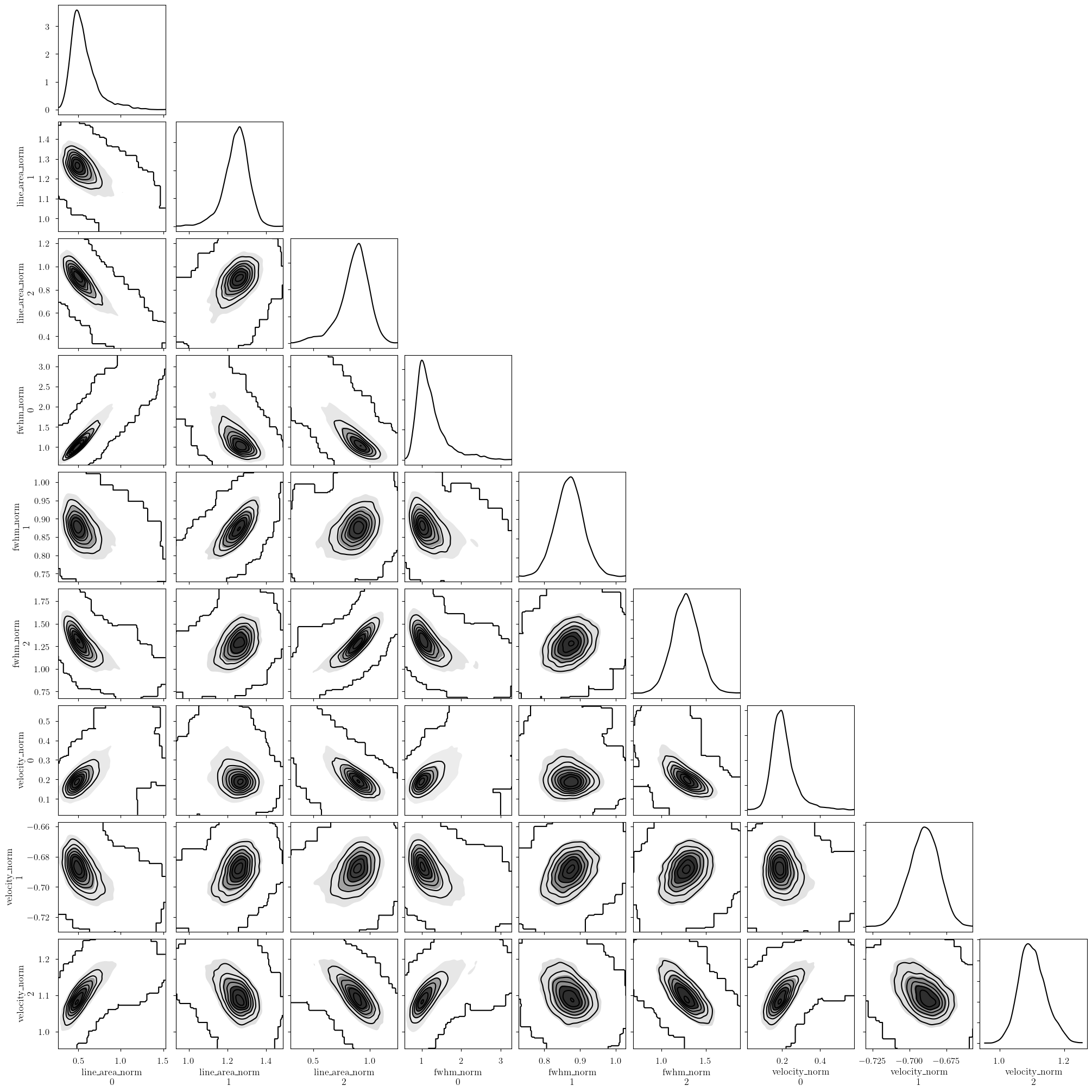
[15]:
_ = plot_pair(
    model.trace.solution_0, # samples
    model.cloud_freeRVs, # var_names to plot
    combine_dims=["cloud"], # concatenate clouds
    labeller=model.labeller, # label manager
    kind="kde", # plot type
    reference_values=sim_params, # truths
)

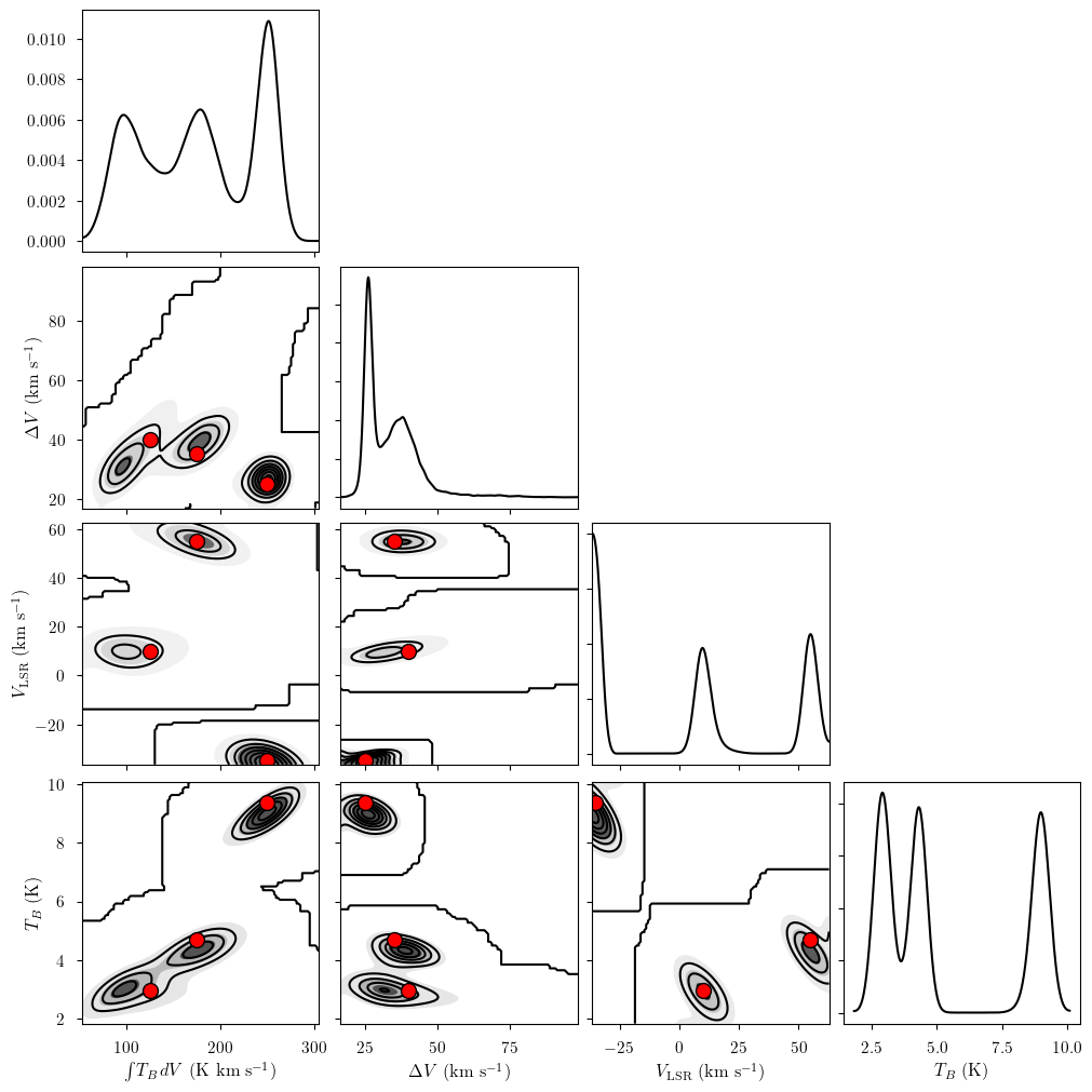
[16]:
_ = plot_pair(
    model.trace.solution_0, # samples
    model.cloud_freeRVs, # var_names to plot
    combine_dims=None, # do not concatenate clouds
    labeller=model.labeller, # label manager
    kind="kde", # plot type
    reference_values=sim_params, # truths
)
[17]:
_ = plot_pair(
    model.trace.solution_0, # samples
    model.cloud_deterministics, # var_names to plot
    combine_dims=["cloud"], # concatenate clouds
    labeller=model.labeller, # label manager
    kind="kde", # plot type
    reference_values=sim_params, # truths
)
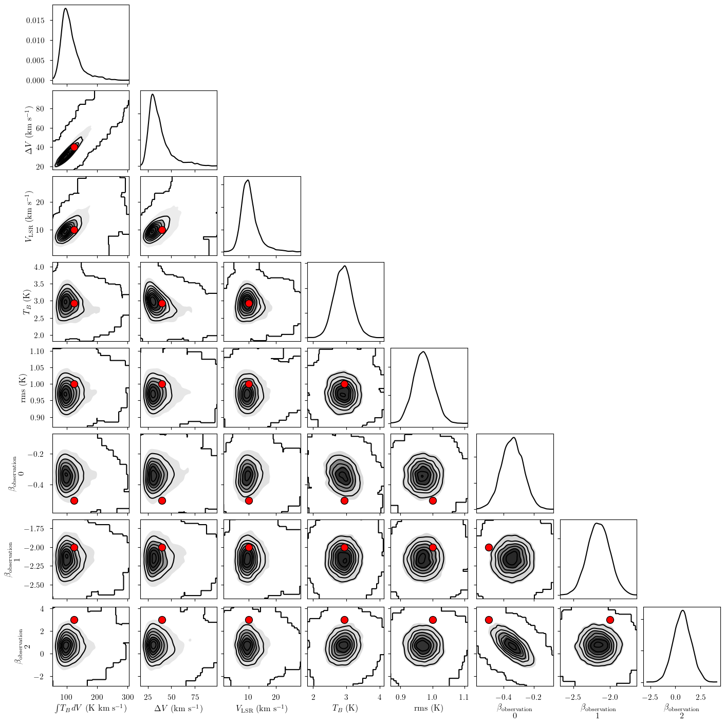
[18]:
my_true_cloud = 1
my_sim_params = {}
for var_name in model.cloud_deterministics:
    my_sim_params[var_name] = sim_params[var_name][my_true_cloud]
for var_name in model.hyper_deterministics:
    my_sim_params[var_name] = sim_params[var_name]
for var_name in model.baseline_freeRVs:
    my_sim_params[var_name] = sim_params[var_name]

_ = plot_pair(
    model.trace.solution_0.sel(cloud=0), # samples
    model.cloud_deterministics + model.hyper_deterministics + model.baseline_freeRVs, # var_names to plot
    labeller=model.labeller, # label manager
    kind="kde", # plot type
    reference_values=my_sim_params, # truths
)
[19]:
point_stats = az.summary(model.trace.solution_0, var_names=model.cloud_deterministics, kind='stats', hdi_prob=0.68)
print("BIC:", model.bic())
point_stats
BIC: 1563.1069404283792
[19]:
| mean | sd | hdi_16% | hdi_84% | |
|---|---|---|---|---|
| line_area[0] | 110.937 | 39.190 | 70.955 | 119.356 |
| line_area[1] | 242.944 | 17.846 | 232.963 | 263.785 |
| line_area[2] | 172.053 | 27.125 | 154.633 | 200.217 |
| fwhm[0] | 39.492 | 16.514 | 22.990 | 41.542 |
| fwhm[1] | 25.164 | 1.315 | 23.860 | 26.399 |
| fwhm[2] | 36.793 | 4.549 | 32.130 | 40.913 |
| velocity[0] | 7.224 | 3.792 | 4.175 | 9.680 |
| velocity[1] | -34.600 | 0.552 | -35.102 | -34.011 |
| velocity[2] | 53.857 | 1.762 | 52.109 | 55.549 |
| amplitude[0] | 2.710 | 0.333 | 2.349 | 3.022 |
| amplitude[1] | 9.067 | 0.438 | 8.758 | 9.534 |
| amplitude[2] | 4.386 | 0.426 | 4.171 | 4.859 |
[ ]: