Basic Tutorial

Trey V. Wenger (c) June 2025

Here we demonstrate the basic features of a bayes_spec model.

# General imports
import numpy as np
import matplotlib.pyplot as plt
import arviz as az
import pandas as pd

print("arviz version:", az.__version__)

import pymc
print("pymc version:", pymc.__version__)

import bayes_spec
print("bayes_spec version:", bayes_spec.__version__)

# Notebook configuration
pd.options.display.max_rows = None

arviz version: 0.22.0dev
pymc version: 5.22.0
bayes_spec version: 1.7.9-staging+2.gb86248c.dirty

Model Definition

First, we define our model. Here we demonstrate a simple Gaussian line profile model where each “cloud” is a set of Gaussian parameters that produces one Gaussian emission line. See the definition of this model in bayes_spec.models.GaussModel, and check out the documentation for guidance on how to create bayes_spec models.

from bayes_spec.models import GaussModel

Data Format

We wish to generate some synthetic data from our model, which requires us to take a brief aside to introduce the bayes_spec data format. We use the SpecData class to pass data into bayes_spec.

from bayes_spec import SpecData

# spectral axis definition
velocity_axis = np.linspace(-250.0, 250.0, 501) # km/s

# data noise can either be a scalar (assumed constant noise across the spectrum)
# or an array of the same length as the data
noise = 1.0 # K

# brightness data. In this case, we just throw in some random data for now
# since we are only doing this in order to simulate some actual data.
brightness_data = noise * np.random.randn(len(velocity_axis)) # K

# Our model only expects a single observation named "observation"
# Note that because we "named" the spectrum "observation" here,
# we must use the same name in the model definition above
observation = SpecData(
    velocity_axis,
    brightness_data,
    noise,
    xlabel=r"Velocity (km s$^{-1}$)",
    ylabel="Brightness Temperature (K)",
)
dummy_data = {"observation": observation}

Simulating Data

Now that we have a model definition and a dummy data format, we can generate simulated observations by drawing samples from the parameter prior distributions.

# Initialize and define the model
n_clouds = 3
baseline_degree = 2
model = GaussModel(dummy_data, n_clouds=n_clouds, baseline_degree=baseline_degree, seed=1234, verbose=True)
model.add_priors(
    prior_line_area = 500.0, # mode of k=2 gamma distribution prior on line area (K km s-1)
    prior_fwhm = 25.0, # mode of k=2 gamma distribution prior on FWHM line width (km s-1)
    prior_velocity = [0.0, 50.0], # mean and width of normal distribution prior on centroid velocity (km s-1)
    prior_baseline_coeffs = [1.0, 1.0, 1.0], # width of normal distribution prior on normalized baseline coefficients
)
model.add_likelihood()

# Draw one posterior predictive sample
simulated = model.sample_prior_predictive(
    samples=1,
)
sim_brightness = simulated.prior_predictive["observation"].sel(chain=0, draw=0).data

# Plot the simulated data
plt.plot(dummy_data["observation"].spectral, sim_brightness, 'k-')
plt.xlabel(dummy_data["observation"].xlabel)
_ = plt.ylabel(dummy_data["observation"].ylabel)

Sampling: [baseline_observation_norm, fwhm_norm, line_area_norm, observation, velocity_norm]

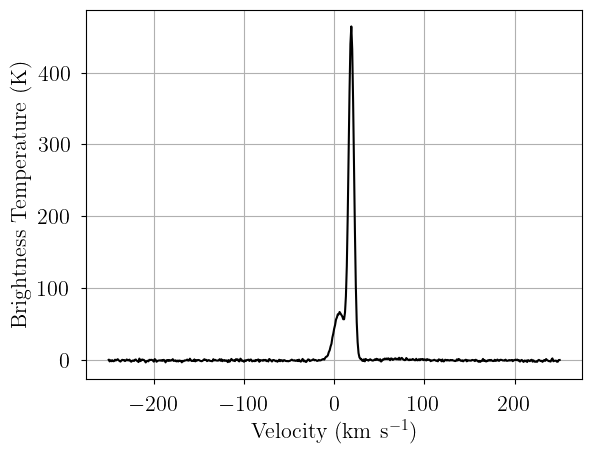
Alternatively, we can pass the relevant parameters directly to the likelihood variable, named observation in our model, to evaluate a model with specific model parameters. Be sure that the simulated values are reasonable given your prior distributions!

sim_params = {
    "fwhm": [25.0, 40.0, 35.0], # FWHM line width (km/s)
    "line_area": [250.0, 125.0, 175.0], # line area (K km/s)
    "velocity": [-35.0, 10.0, 55.0], # velocity (km/s)
    "baseline_observation_norm": [-0.5, -2.0, 3.0], # normalized baseline coefficients
}

# add derived quantities to sim_params
for key in model.cloud_deterministics:
    if key not in sim_params.keys():
        sim_params[key] = model.model[key].eval(sim_params, on_unused_input="ignore")

# Evaluate and save simulated observation
sim_brightness = model.model.observation.eval(sim_params, on_unused_input="ignore")

# Plot the simulated data
plt.plot(dummy_data["observation"].spectral, sim_brightness, 'k-')
plt.xlabel(dummy_data["observation"].xlabel)
_ = plt.ylabel(dummy_data["observation"].ylabel)

sim_params

{'fwhm': [25.0, 40.0, 35.0],
 'line_area': [250.0, 125.0, 175.0],
 'velocity': [-35.0, 10.0, 55.0],
 'baseline_observation_norm': [-0.5, -2.0, 3.0],
 'amplitude': array([9.39437279, 2.9357415 , 4.69718639])}

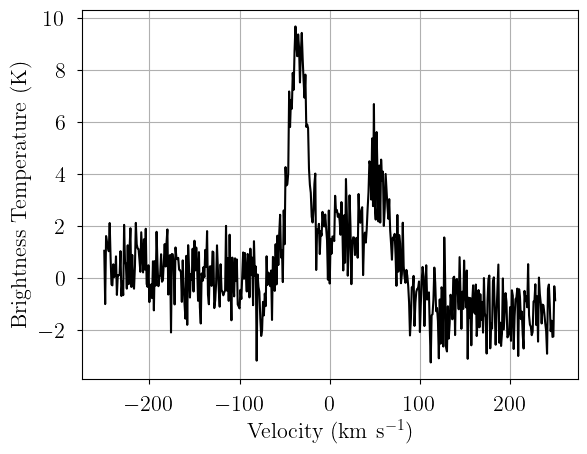
# Now we pack the simulated spectrum into a new SpecData instance
observation = SpecData(
    velocity_axis,
    sim_brightness,
    noise,
    xlabel=r"Velocity (km s$^{-1}$)",
    ylabel="Brightness Temperature (K)",
)
data = {"observation": observation}

Model

Finally, with our model definition and (simulated) data in hand, we can explore the capabilities of bayes_spec.

We begin with a three-cloud (n_cloud=3) model, with a 2nd order polynomial baseline (baseline_degree=2). Each “cloud” is a set of Gaussian parameters that produces a single Gaussian emission line. The length of prior_baseline_coeffs must be baseline_degree + 1, and generally can be left at the default value since the data and baseline are internally normalized.

model = GaussModel(data, n_clouds=n_clouds, baseline_degree=baseline_degree, seed=1234, verbose=True)
model.add_priors(
    prior_line_area = 500.0, # mode of k=2 gamma distribution prior on line area (K km s-1)
    prior_fwhm = 25.0, # mode of k=2 gamma distribution prior on FWHM line width (km s-1)
    prior_velocity = [0.0, 50.0], # mean and width of normal distribution prior on centroid velocity (km s-1)
    prior_baseline_coeffs = [1.0, 1.0, 1.0], # width of normal distribution prior on normalized baseline coefficients
)
model.add_likelihood()

# Plot model graph
model.graph()

The model graph shows the relationship between the free parameters (ellipses), derived quantities (rectangles), and observed data (filled ellipses). Each “group” or “box” describes groups of parameters or values with a specific dimension: since baseline_degree=2 then baseline_coeff has length 3, since n_clouds=3 the number of clouds is 3, and there are 501 data points (channels) in our spectrum (observation).

# model string representation
print(model.model.str_repr())

baseline_observation_norm ~ Normal(0, <constant>)
           line_area_norm ~ Gamma(2, f())
                fwhm_norm ~ Gamma(2, f())
            velocity_norm ~ Normal(0, 1)
                line_area ~ Deterministic(f(line_area_norm))
                     fwhm ~ Deterministic(f(fwhm_norm))
                 velocity ~ Deterministic(f(velocity_norm))
                amplitude ~ Deterministic(f(fwhm_norm, line_area_norm))
              observation ~ Normal(f(fwhm_norm, line_area_norm, baseline_observation_norm, velocity_norm), <constant>)

We check that our prior distributions are reasonable by drawing prior predictive checks. Each colored line is a simulated “observation” with parameters drawn from the prior distributions. You should check that these simulated observations at least somewhat overlap your actual observation (black line).

from bayes_spec.plots import plot_predictive

# prior predictive check
prior = model.sample_prior_predictive(
    samples=1000,  # prior predictive samples
)
_ = plot_predictive(model.data, prior.prior_predictive)

Sampling: [baseline_observation_norm, fwhm_norm, line_area_norm, observation, velocity_norm]

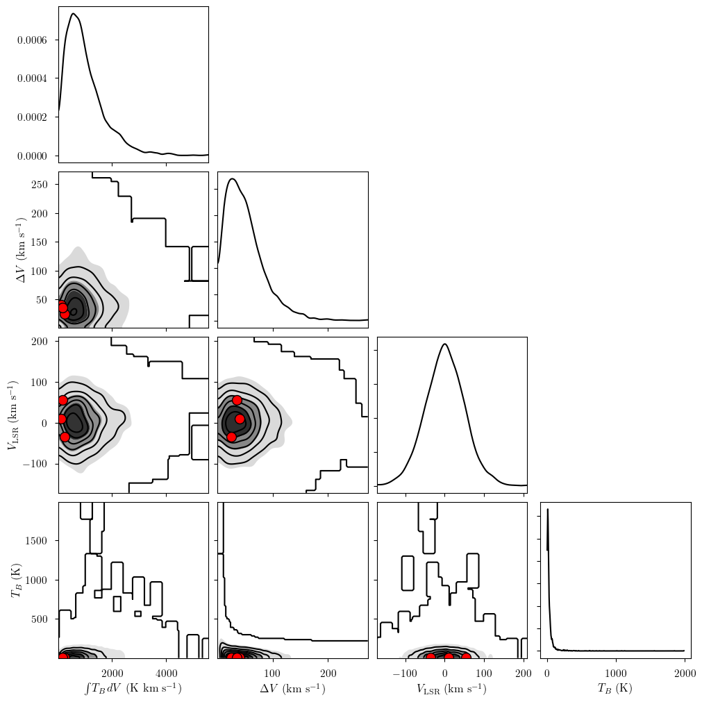
We can also generate a pair plot to inspect the prior distributions and their effect on deterministic quantities. The model has several attributes to access the various free parameters (freeRVs) and deterministic quantities (deterministics). Here we show the pair plot for the deterministic quantities derived from our prior distributions. The three red points correspond to the simulation parameters (“truths”) for our three clouds.

from bayes_spec.plots import plot_pair

# available parameter attributes:
print("baseline_freeRVs", model.baseline_freeRVs)
print("baseline_deterministics", model.baseline_deterministics)
print("cloud_freeRVs", model.cloud_freeRVs)
print("cloud_deterministics", model.cloud_deterministics)
print("hyper_freeRVs", model.hyper_freeRVs)
print("hyper_deterministics", model.hyper_deterministics)

_ = plot_pair(
    prior.prior, # samples
    model.cloud_deterministics, # var_names to plot
    combine_dims=["cloud"], # concatenate clouds
    labeller=model.labeller, # label manager
    kind="kde", # plot type
    reference_values=sim_params, # truths
)

baseline_freeRVs ['baseline_observation_norm']
baseline_deterministics []
cloud_freeRVs ['line_area_norm', 'fwhm_norm', 'velocity_norm']
cloud_deterministics ['line_area', 'fwhm', 'velocity', 'amplitude']
hyper_freeRVs []
hyper_deterministics []

Posterior Sampling: Variational Inference

We can approximate the posterior distribution using variational inference (VI). We will run a maximum of n iterations, but stop early if it appears that VI has converged on a solution. You will have to tune the convergence thresholds and learning rate for your model. We help the sampler along by initializing the velocity parameter over the range of the prior.

model.fit(
    n = 100_000, # maximum number of VI iterations
    draws = 1_000, # number of posterior samples
    rel_tolerance = 0.01, # VI relative convergence threshold
    abs_tolerance = 0.05, # VI absolute convergence threshold
    learning_rate = 1e-2, # VI learning rate
    start = {"velocity_norm": np.linspace(-3.0, 3.0, n_clouds)},
)

Convergence achieved at 5400
Interrupted at 5,399 [5%]: Average Loss = 1,995.4

Adding log-likelihood to trace

# posterior samples stored in model.trace.posterior
az.summary(model.trace.posterior)

arviz - WARNING - Shape validation failed: input_shape: (1, 1000), minimum_shape: (chains=2, draws=4)

	mean	sd	hdi_3%	hdi_97%	mcse_mean	mcse_sd	ess_bulk	ess_tail	r_hat
baseline_observation_norm[0]	-0.481	0.045	-0.570	-0.399	0.001	0.001	995.0	906.0	NaN
baseline_observation_norm[1]	-1.996	0.155	-2.289	-1.715	0.005	0.004	950.0	967.0	NaN
baseline_observation_norm[2]	0.333	0.675	-0.932	1.635	0.023	0.014	853.0	944.0	NaN
velocity_norm[0]	0.121	0.036	0.055	0.188	0.001	0.001	1029.0	814.0	NaN
velocity_norm[1]	-0.702	0.007	-0.717	-0.690	0.000	0.000	970.0	926.0	NaN
velocity_norm[2]	1.075	0.019	1.037	1.108	0.001	0.000	909.0	790.0	NaN
line_area_norm[0]	0.211	0.017	0.181	0.243	0.001	0.000	786.0	799.0	NaN
line_area_norm[1]	0.462	0.012	0.440	0.483	0.000	0.000	998.0	892.0	NaN
line_area_norm[2]	0.337	0.016	0.310	0.368	0.001	0.000	889.0	906.0	NaN
fwhm_norm[0]	1.645	0.155	1.363	1.953	0.005	0.004	829.0	733.0	NaN
fwhm_norm[1]	0.943	0.029	0.895	0.998	0.001	0.001	931.0	941.0	NaN
fwhm_norm[2]	1.440	0.072	1.312	1.582	0.002	0.002	916.0	906.0	NaN
line_area[0]	105.566	8.430	90.447	121.329	0.301	0.220	786.0	799.0	NaN
line_area[1]	231.011	5.869	219.997	241.586	0.185	0.139	998.0	892.0	NaN
line_area[2]	168.438	7.782	154.879	183.944	0.260	0.182	889.0	906.0	NaN
fwhm[0]	41.118	3.867	34.065	48.830	0.135	0.088	829.0	733.0	NaN
fwhm[1]	23.564	0.717	22.367	24.945	0.023	0.015	931.0	941.0	NaN
fwhm[2]	36.001	1.803	32.788	39.545	0.059	0.040	916.0	906.0	NaN
velocity[0]	6.048	1.802	2.749	9.395	0.056	0.041	1029.0	814.0	NaN
velocity[1]	-35.120	0.370	-35.848	-34.476	0.012	0.009	970.0	926.0	NaN
velocity[2]	53.731	0.949	51.870	55.413	0.031	0.022	909.0	790.0	NaN
amplitude[0]	2.433	0.300	1.868	2.946	0.010	0.009	941.0	992.0	NaN
amplitude[1]	9.218	0.372	8.523	9.906	0.012	0.008	910.0	867.0	NaN
amplitude[2]	4.407	0.303	3.842	4.961	0.010	0.007	1005.0	1023.0	NaN

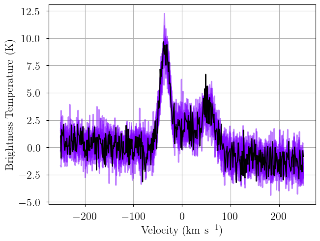
It’s good practice to verify the integrity of your solution! Here we generate posterior predictive checks – realizations of the model drawn with parameters drawn from the posterior distribution. Each line is one posterior sample.

posterior = model.sample_posterior_predictive(
    thin=100, # keep one in {thin} posterior samples
)
_ = plot_predictive(model.data, posterior.posterior_predictive)

Sampling: [observation]

Posterior Sampling: MCMC

VI is fast, but it’s not particularly accurate, and there is no way to diagnose “convergence”. Instead, we sample the posterior distribution using MCMC. Here we initialize the No U-Turn Sampler (NUTS) using VI (also available is the pymc default: init="jitter+adapt_diag", which may be better suited to some models). We can customize the VI initialization as well as the NUTS parameters. If there are many divergences, or if the resulting effective sample sizes are small and r_hat is large, try increasing the number of tuning samples, draws, and/or chains. Increasing target_accept to 0.9 or 0.95 can help if there are many divergences. Use as many chains as possible.

init_kwargs = {
    "rel_tolerance": 0.01,
    "abs_tolerance": 0.01,
    "learning_rate": 0.001,
    "start": {"velocity_norm": np.linspace(-3.0, 3.0, model.n_clouds)},
}
model.sample(
    init = "advi+adapt_diag", # initialization strategy
    tune = 1000, # tuning samples
    draws = 1000, # posterior samples
    chains = 8, # number of independent chains
    cores = 8, # number of parallel chains
    init_kwargs = init_kwargs, # VI initialization arguments
    nuts_kwargs = {"target_accept": 0.8}, # NUTS arguments
)

Initializing NUTS using custom advi+adapt_diag strategy

Convergence achieved at 23200
Interrupted at 23,199 [2%]: Average Loss = 3,788.9
Multiprocess sampling (8 chains in 8 jobs)
NUTS: [baseline_observation_norm, line_area_norm, fwhm_norm, velocity_norm]

Sampling 8 chains for 1_000 tune and 1_000 draw iterations (8_000 + 8_000 draws total) took 6 seconds.

Adding log-likelihood to trace

There were 1 divergences in converged chains.

If a chain does not converge, an error is printed and that chain is dropped from all subsequent analyses. In the remaining chains, there may be some divergences. The number of divergences should be much less than the number of posterior samples.

In general, there could be a labeling degeneracy, or multiple unique solutions. Here we “solve” for those effects using a Gaussian Mixture Model (GMM). The parameter kl_div_threshold defines the probability threshold for “unique” GMM solutions.

model.solve(kl_div_threshold=0.1)

GMM converged to unique solution
Label order mismatch in solution 0
Chain 0 order: [0 1 2]
Chain 1 order: [0 1 2]
Chain 2 order: [0 1 2]
Chain 3 order: [0 1 2]
Chain 4 order: [0 1 2]
Chain 5 order: [2 1 0]
Chain 6 order: [0 1 2]
Chain 7 order: [0 1 2]
Adopting (first) most common order: [0 1 2]

print("solutions:", model.solutions)
display(az.summary(model.trace["solution_0"]))
# this also works: az.summary(model.trace.solution_0)

solutions: [0]

	mean	sd	hdi_3%	hdi_97%	mcse_mean	mcse_sd	ess_bulk	ess_tail	r_hat
baseline_observation_norm[0]	-0.488	0.072	-0.622	-0.350	0.001	0.001	5369.0	5506.0	1.0
baseline_observation_norm[1]	-1.982	0.155	-2.266	-1.684	0.002	0.002	8018.0	4386.0	1.0
baseline_observation_norm[2]	0.421	0.897	-1.284	2.058	0.011	0.009	6523.0	5486.0	1.0
velocity_norm[0]	0.140	0.107	-0.062	0.358	0.002	0.002	2719.0	2503.0	1.0
velocity_norm[1]	-0.705	0.009	-0.722	-0.688	0.000	0.000	4674.0	5175.0	1.0
velocity_norm[2]	1.097	0.031	1.039	1.153	0.001	0.000	3281.0	5162.0	1.0
line_area_norm[0]	0.289	0.081	0.153	0.434	0.002	0.001	1775.0	2970.0	1.0
line_area_norm[1]	0.433	0.036	0.368	0.496	0.001	0.000	2449.0	4351.0	1.0
line_area_norm[2]	0.297	0.052	0.195	0.388	0.001	0.001	1936.0	2250.0	1.0
fwhm_norm[0]	2.300	0.672	1.160	3.477	0.016	0.007	1832.0	3117.0	1.0
fwhm_norm[1]	0.907	0.051	0.807	0.999	0.001	0.001	3210.0	5023.0	1.0
fwhm_norm[2]	1.368	0.156	1.084	1.680	0.003	0.002	2832.0	2891.0	1.0
line_area[0]	144.585	40.257	76.542	216.880	0.960	0.525	1775.0	2970.0	1.0
line_area[1]	216.319	17.780	184.071	248.036	0.359	0.167	2449.0	4351.0	1.0
line_area[2]	148.517	26.209	97.343	194.236	0.616	0.391	1936.0	2250.0	1.0
fwhm[0]	57.494	16.796	29.011	86.929	0.393	0.184	1832.0	3117.0	1.0
fwhm[1]	22.671	1.282	20.187	24.979	0.023	0.013	3210.0	5023.0	1.0
fwhm[2]	34.212	3.898	27.100	41.994	0.073	0.049	2832.0	2891.0	1.0
velocity[0]	6.994	5.375	-3.124	17.917	0.108	0.107	2719.0	2503.0	1.0
velocity[1]	-35.243	0.454	-36.090	-34.386	0.007	0.005	4674.0	5175.0	1.0
velocity[2]	54.829	1.532	51.939	57.633	0.027	0.016	3281.0	5162.0	1.0
amplitude[0]	2.385	0.227	1.971	2.815	0.003	0.002	6568.0	6357.0	1.0
amplitude[1]	8.959	0.444	8.109	9.749	0.007	0.004	3729.0	6171.0	1.0
amplitude[2]	4.062	0.457	3.178	4.842	0.010	0.006	2486.0	3212.0	1.0

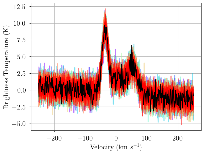
We again generate posterior predictive checks as well as a trace plot of the individual chains. Each line is one posterior sample.

posterior = model.sample_posterior_predictive(
    thin=100, # keep one in {thin} posterior samples
)
_ = plot_predictive(model.data, posterior.posterior_predictive)

Sampling: [observation]

from bayes_spec.plots import plot_traces

axes = plot_traces(model.trace.solution_0, model.cloud_freeRVs + model.baseline_freeRVs + model.hyper_freeRVs)
fig = axes.ravel()[0].figure
fig.tight_layout()

In these trace plots, each linestyle represents a different Markov chain (there are four different chains and linestyles), and each color represents a different parameter group. For example, there are three colors for line_area_norm representing the three clouds of the model, and there are three colors for baseline_observation_norm representing the three baseline coefficients (since baseline_degree=2 there are three polynomial baseline coefficients).

We can inspect the posterior distribution pair plots. First, the free cloud parameters.

_ = plot_pair(
    model.trace.solution_0, # samples
    model.cloud_freeRVs, # var_names to plot
    combine_dims=["cloud"], # concatenate clouds
    labeller=model.labeller, # label manager
    kind="kde", # plot type
    reference_values=sim_params, # truths
)

Notice that there are three posterior modes. These correspond to the three clouds of the model. We can plot each cloud against the other to see degeneracies between clouds.

_ = plot_pair(
    model.trace.solution_0, # samples
    model.cloud_freeRVs, # var_names to plot
    combine_dims=None, # do not concatenate clouds
    labeller=model.labeller, # label manager
    kind="kde", # plot type
    reference_values=sim_params, # truths
)

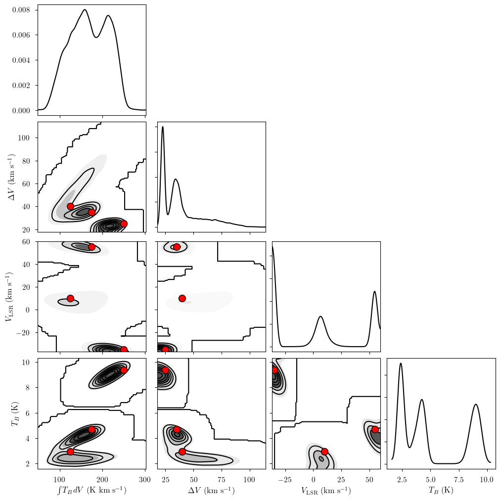
And the cloud deterministic quantities.

_ = plot_pair(
    model.trace.solution_0, # samples
    model.cloud_deterministics, # var_names to plot
    combine_dims=["cloud"], # concatenate clouds
    labeller=model.labeller, # label manager
    kind="kde", # plot type
    reference_values=sim_params, # truths
)

We can plot the posterior distributions for a single cloud.

my_true_cloud = 1
my_sim_params = {}
for var_name in model.cloud_deterministics:
    my_sim_params[var_name] = sim_params[var_name][my_true_cloud]
for var_name in model.baseline_freeRVs:
    my_sim_params[var_name] = sim_params[var_name]

_ = plot_pair(
    model.trace.solution_0.sel(cloud=0), # samples
    model.cloud_deterministics + model.baseline_freeRVs, # var_names to plot
    labeller=model.labeller, # label manager
    kind="kde", # plot type
    reference_values=my_sim_params, # truths
)

Finally, we can get the posterior statistics, Bayesian Information Criterion (BIC), etc.

point_stats = az.summary(model.trace.solution_0, var_names=model.cloud_deterministics, kind='stats', hdi_prob=0.68)
print("BIC:", model.bic())
point_stats

BIC: 1435.1845464712758

	mean	sd	hdi_16%	hdi_84%
line_area[0]	144.585	40.257	95.192	174.480
line_area[1]	216.319	17.780	199.338	236.426
line_area[2]	148.517	26.209	125.620	176.573
fwhm[0]	57.494	16.796	35.164	69.854
fwhm[1]	22.671	1.282	21.427	23.979
fwhm[2]	34.212	3.898	30.796	38.257
velocity[0]	6.994	5.375	1.969	11.263
velocity[1]	-35.243	0.454	-35.703	-34.813
velocity[2]	54.829	1.532	53.253	56.309
amplitude[0]	2.385	0.227	2.154	2.595
amplitude[1]	8.959	0.444	8.574	9.472
amplitude[2]	4.062	0.457	3.786	4.638